How To Set Up Headers In Excel

Column Header in Excel (Table of Contents)

Introduction to Column Header in Excel
How to Use Column Header in Excel?

Column Header is a very important part of excel as we work on dissimilar types of Tables in excel every 24-hour interval. Column Headers basically tell us the category of the data in that column to which it belongs. For example, if column A contains Engagement, and so Column header for Cavalcade A will be "Date", or suppose column B contains Names of the pupil, then column header for Column B volition be "Educatee Proper name". Cavalcade Headers are of import in a manner when a new person looks at your excel; he can understand the meaning of the data in those columns. It is as well important because yous need to call up how the data has been organized in your excel. And then from the data organization standpoint, Column Headers play a very important function.

In this article, we volition look at the best possible ways of how nosotros can organize or format the column headers in excel. There are many ways of creating headers in excel. The three best possible ways of creating headers are beneath.

Freezing Row/Column.
Printing a header row.
Creating a header in Table.

Nosotros will look at each manner of creating a header one by one with the help of examples.

Suppose you are working on the data which has a large number of rows, and when you scroll downwardly in the worksheet to expect at some data, you may non be able to wait at the Cavalcade Header. This is where Freeze Panes helps in excel. You lot can gyre down in the excel canvass without losing visibility to the column headers.

How to Use Column Header in Excel?

Column Header in Excel is very simple and like shooting fish in a barrel. Allow'due south understand how to use the column Header in Excel with some examples.

Y'all can download this Column Header Excel Template here – Column Header Excel Template

Case #one – Freezing Row/Column

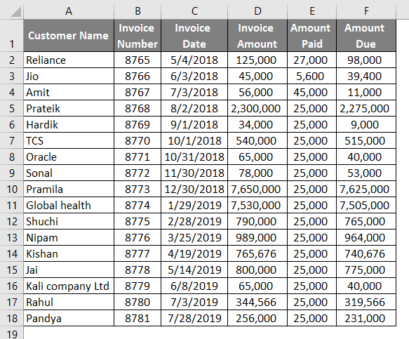
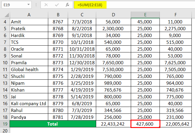
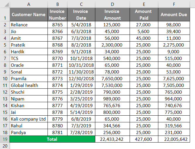
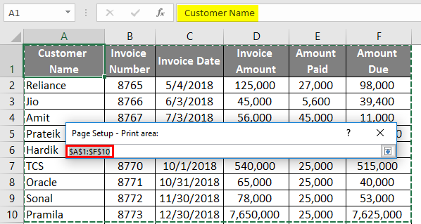
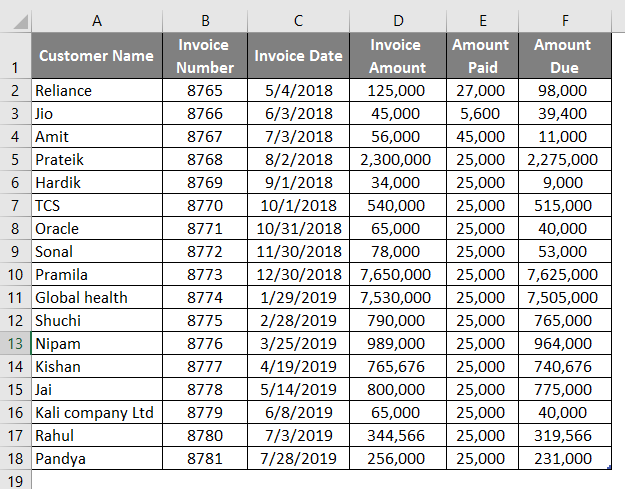
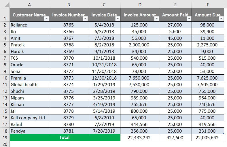
Suppose at that place is information related to customers in excel, every bit shown in the below screenshot.

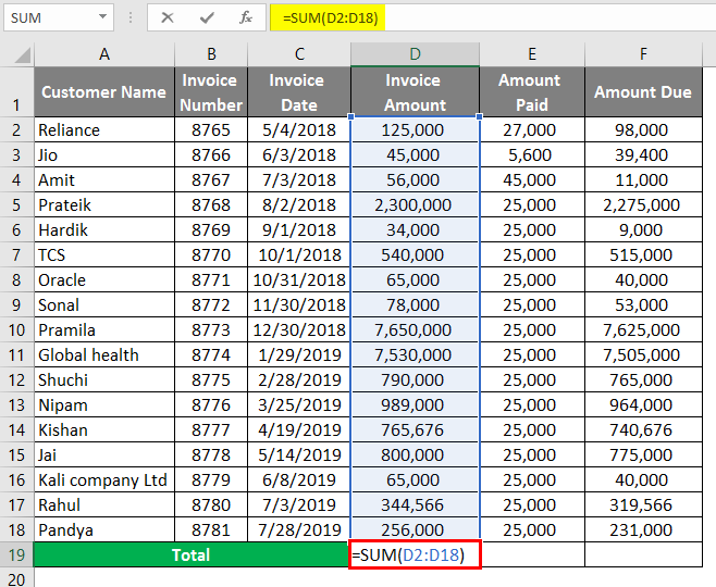
Use SUM formula in cell D19.

After using the SUM formula, the output is shown beneath.

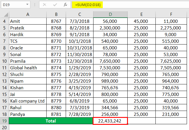
The same formula is used in prison cell E19 and cell F19.

You need to follow the below steps to freeze the superlative row.

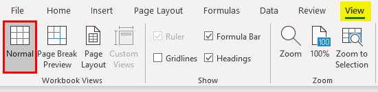
Get to the View tab in Excel.

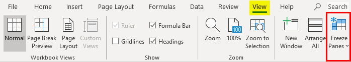
Click on the Freeze Pane Choice

You will come across three options afterward clicking on the Freeze Pane choice. Y'all demand to select the "Freeze Top Row" option.

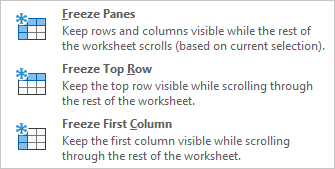
In one case you click on the "Freeze Acme Row", the top row will be freezer, and yous scroll downward in excel without losing visibility to excel. You lot tin can run into in the below screenshot that Row 1, which has column headers, are still visible even when you scroll down.

Example #2 – Printing a Header Row

When you lot are working on large spreadsheets where data is spread across multiple pages and when you need to take a print out, it doesn't fit well on one page. The printing job becomes frustrating as yous are non able to see the cavalcade headers in impress afterward the first page. In that scenario, there is a functionality in excel known every bit "Print Titles", which helps gear up a row or rows to print at the top of every folio. We will accept a like example which we accept taken in Example 1.

Follow the beneath steps to employ this functionality in Excel.

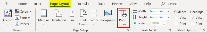
Get to the Page Layout tab in Excel.

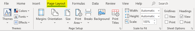
Click on Print Titles.

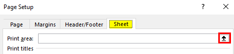
Afterwards clicking on the Impress Titles option, you will see the below window open for Page Fix in excel.

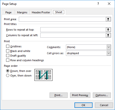
In the Page Gear up window, y'all will observe different options that you tin can choose.

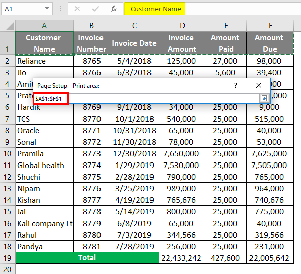
(a) Print Area

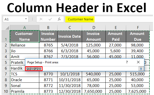
To select Print Surface area, click on the button on the right side, as shown in the screenshot.

Later clicking on the button, the navigation window will open. You can select from Row 1 to Row 10 to print the first 10 rows.

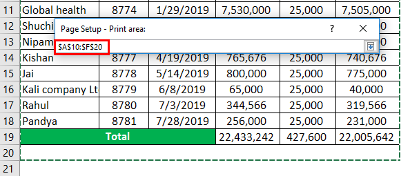
If you want to impress Row 11 to Row 20, you can select the Impress Surface area as Row 11 to Row 20.

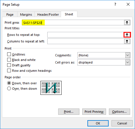
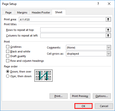
Under Print Titles, you tin can find two options.

(b) Rows to Repeat at Top

This is where we demand to select the column header, which we desire to echo on every page of the printout. To select Rows to repeat at the top, click on the push button on the right side, equally shown in the screenshot.

After clicking on the push button, the navigation window volition open. You can select Row i, as shown in the below screenshot.

(C) Columns to Repeat at Left

This is the cavalcade that you desire to encounter on the left, which will repeat on every page. We volition proceed it as blank as we don't have any row headers in our tabular array.

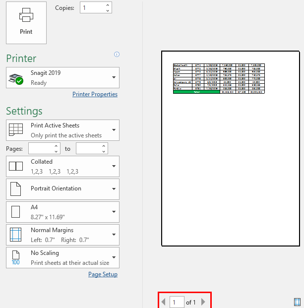
Now click on the "Print Preview" selection on the page setup as shown in the below screenshot to see the Print Preview. As you can come across in the below screenshot, the print area is from Row 11 to Row 20, with the column headers in Row 1.

Click on Ok in the Page setup window after exiting from Print Preview.

Case #3 – Creating a Header in a Tabular array

One of the features in Excel is that you can convert your information into a Table. Information technology automatically creates Headers when y'all convert your information into a table. Just please take a note here that these headers are dissimilar from the Worksheet column heading or printed headers which nosotros have seen earlier.

We will take a like example which we accept taken earlier.

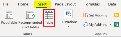
Click on the "Insert" tab and then click on the "Table" push.

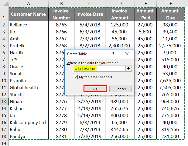
Later clicking on the "Table" option, you can requite the range of information that you desire to convert into the table and also select the checkbox of "My Table has Headers", as shown in the below screenshot. The first row of your selection will automatically be assigned equally column headers.

Click Ok. You will encounter your data is converted into a Table.

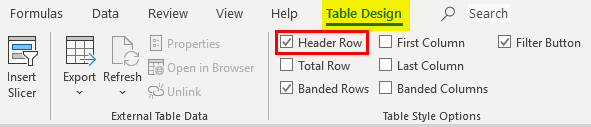
You can Enable or Disable the Header row past going into the "Design" tab of the Table.

Things to Recall About Column Headers in Excel

Always remember to format column headers differently and use Freeze panes to have visibility on the cavalcade header at all times. It will aid you save time of scrolling up and down to empathise data.
Make sure to use the Print Area pick and Rows to echo at every folio choice while printing. This will make your printing job piece of cake.
Selection of Range and Column header is important while creating Table in Excel.

Recommended Commodity

This is a guide to Cavalcade Header in Excel. Here we discuss How to apply Cavalcade Header in Excel along with practical examples and downloadable excel template. You can also go through our other suggested articles –

Compare Two Columns in Excel for Matches
Freeze Columns in Excel
COLUMNS Formula in Excel
Excel Header Row